As described in our TechNote „Linearization“, it is an important task to linearize digital images before any calculations can be done.
Just to remember: For example, if you analyze gamma corrected images in case of resolution measurement, the output data regarding to the reflectance won’t be linear (but should be for analysis)¹.
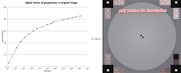
Figure 1 shows a sinusoidal Siemens star with 16 gray patches. The diagram shows the relationship between the reflectance of the patches and the digital values (DV) in the image. For linearization you can use the inverse function to map the original values to a straight line.

Figure 1. sinusodial Siemens star in original image
So if you want to linearize the opto-electronical conversion function (OECF) depicted above, you have at least three different methods to do so. We call them:
- Full Image Range
- Modulation Transfer Function (MTF)
- Full Data Range

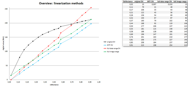
Figure 2. Overview: linearization methods
1) Full Image Range
The first attempt to linearize images is that we decide to choose the minimum digital value² in the image as our reference black and the maximum DV as reference white. With these two points we can determine a straight line to map the original DVs to equivalent points on this line. We call this method ‘Full Image Range’ because we’re using the highest and lowest values within the image. In Figure 2 you can see the green line starting at the minimum DV going up to the maximum DV in the original image.
2) Modulation transfer function (MTF)
The ‘MTF’ and ‘Full Image Range’ methods are very similar, except that the ‘MTF’ has an additional offset of

in order to map the lowest incoming value to zero. As you can see in Figure 2, the blue line (MTF) and the green line (Full Image Range) have the same slope, but a different offset in the linear equation and this offset is the minimum value in the original image (taken from the black patch). So the range of this ‘MTF’ method’s straight line will be

3) Full Data Range
If you want to use the full bit-depth of an image from zero to the highest value you can get, you can map the original data to a straight line going from

This method is represented by the red line in Figure 2.
All methods have one thing in common: You always define two reference points and calculate a linear equation to map the original values to. But one thing is different between the ‘Full Data Range’ / ‘MTF’ and the ‘Full Image Range’ method regarding to the contrast:
With the values shown in the table (Figure 2) and the following equation

the first two methods provide a contrast of one (as they use zero as minimum signal), but the ‘Full Image Range’ method has the same contrast like the original image.

The decision of using one of the above mentioned methods depends on the field of application.
For example if you want to determine noise (as standard deviation) in the darkest/lightest region of your image, it may be a problem if you use the ‘Full Data Range’ or ‘MTF’ method due to clipping. But if a contrast of one is needed, you can use the ‘MTF’ or ‘Full Data Range’ method, as you can see in the table in Figure 3.
________________________________
¹See ‚Linearization‘ TechNote for further details
²In the following, minimum and maximum digital values refer to the mean values of the darkest and brightest patch in the image.
ck

